Geospatial Analytics – from Retrospective to Predictive and Why You Should Care?
Asset and construction monitoring has evolved at an arguably slow pace over the past few centuries. While very rare today to see a level and staff being manually used to determine the height difference between two points, it is still common to see a Total Station being used for the same purpose – a machine that has been around since the early 1970s. Both of these devices rely on principles devised by the ancient Greeks – while the hardware has of course progressed, the basic calculations have not.
What has evolved significantly faster though is our ability to interpret results from these data-capture devices and more importantly, make better meaning of the data converting it into knowledge that can then be used for purposes such as asset behavior diagnostics.
In conjunction, today we live in a world where data capture isn’t our bottleneck anymore either – it’s the complete opposite – vast volumes of data are captured both manually and automatically that then require interpretation and analysis. In the past twenty years, computing power has helped with this challenge.
As a result of this, geospatial platforms are now moving away from simple displaying of raw data to advanced interpretation of data. However, this is still a stepping stone. Most analysis focuses on the retrospective i.e., interpreting asset behavior in the past. But what about looking beyond the past? What if we could use historical behavioral patterns to better help predict the future state of an asset? Modeling when an asset may fail or better still, determination of the most appropriate time for maintenance investment.
Retrospective Geospatial Analysis
One of the hardest challenges with analyzing geospatial data is trying to determine what the data is really telling you. Looking at a time-series of say vertical movement of an asset that contains thousands and thousands of points over time requires human patience. Fortunately, this can be augmented by some basic computing power.
Algorithms exist today that can help quickly remove noise from large data sets. Figure 1 shows an example of a time-series movement chart for an asset over a 6-year period. As an analyst, I must spend time and effort trying to manually interpret this noisy and complex line.
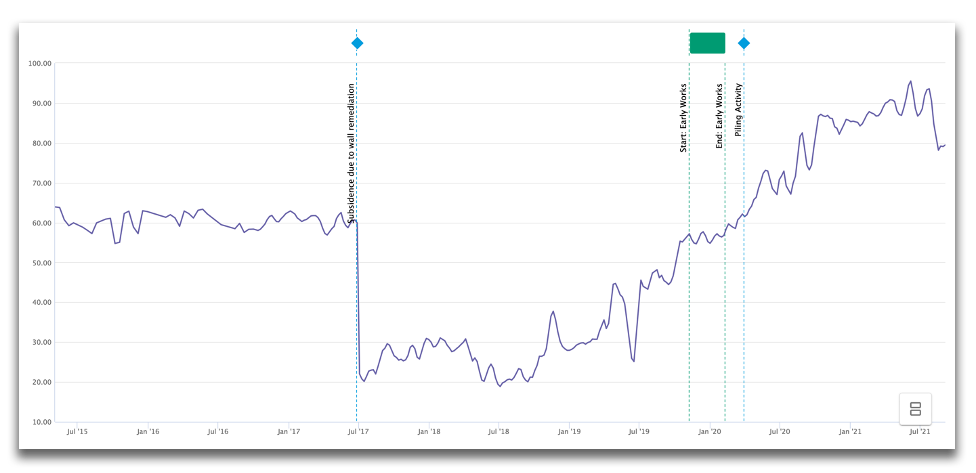
Figure 1 – 6 Year Time Series Line
To help me with the interpretation of this large dataset, I can apply a smoothing algorithm that reduces the noise and drives insight towards bigger picture trends over time. This is extremely helpful as it then gives me insight into trend variation without being skewed by local noise or abnormalities.
In the example below, I can see there is a downward trend up until July 2018 and then a reverse upward trend in the vertical movement of the asset in question.
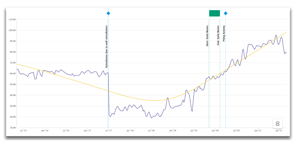
Figure 2 – Trend-Change Determination
Such trend determination is helpful when considering drivers such as climate change and other long-term influencers but what about insight into shorter-term influencers? This becomes even more important during the construction phase of an asset where there can be influence changes on a daily or even hourly basis.
In the same way, we can determine long-term trend change, we can also use simple algorithms to determine short-term step changes.
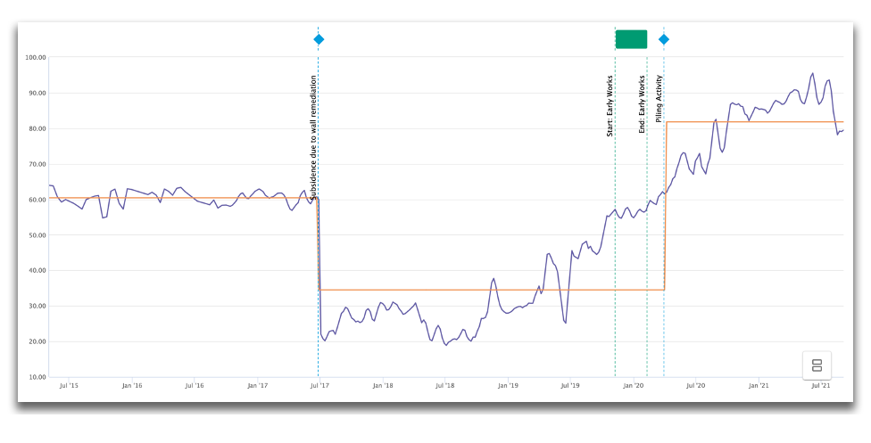
Figure 3 – Short-Term Step-Change Detection
In Figure 3 above, the computer has identified two points in time where there are discrete changes in asset height. These changes are not necessarily associated with the bigger-picture trend change. The first is the result of an adjacent asset failure – a wall failure that had a material impact on the asset. The second is because of a different root cause – construction itself. By overlaying the construction schedule, the analyst is able to pinpoint piling activities that occurred at the exact same time as the asset shift. From this, it can be determined, with a high degree of certainty, that the construction piling activities were the cause of the shift in asset height in early 2020.
Such root cause determination is possible due to the overlay of different dimensions – in this example, the asset movement and a construction schedule. However, the actual determination of the root cause (or correlation between the piling event and the asset movement event) is still largely down to the analyst’s expertise but even that responsibility is changing…
Today, mathematical correlation is being used to automatically determine relationships between assets and their environmental drivers such as construction activities. Analysts are being handed more and more guidance giving them more time to focus their expertise on making smart decisions rather than spending their time simply interpreting the data.
The real value of these advancements, however, is in the determination of the future state. We are on the cusp of being able to truly predict the future…
Predictive Geospatial Analysis
With the help of historical behavioral smoothing, trend detection, and discrete point-in-time change detection, we are becoming more proficient in being able to more accurately forecast future states through the use of extrapolation techniques.
There are numerous extrapolation techniques both algorithmic and statistical, and few of these are new. Table 1 below shows some examples of these.
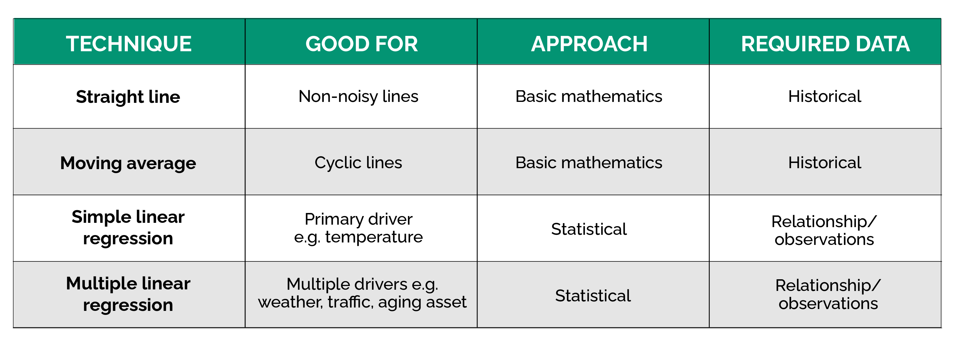
Table 1 – Algorithmic Forecasting Techniques
What is key though is none are necessarily better than the other. At the end of the day, a forecast is just a model of future state. If our asset movement over time is linear, then a straight-line extrapolation technique is appropriate; if the asset movement cycles over time, then better to adopt more of a moving average type approach. If there are multiple influences that are known to have a material impact on the asset, then we should consider more of a multiple linear regression approach. We need to apply an appropriate forecasting technique to fit the historical behavior of the asset!
There is not a shortage of mathematical or statistical based approaches available at our fingertips. Again, that’s not our real challenge. Our real challenge is to figure out which forecasting technique is most appropriate for the asset in question. To best achieve this, we need to firstly re-visit the historical behavior and better understand the patterns to date to help us make a better forecasting choices. This is where machine learning and AI can have a real impact.
BKwai’s data science team have been developing technology to automate this forecasting selection process. As such, the ability to forecast more accurately is now a reality.
By looking across multiple assets, the most frequent root cause of historical behavior can start to be determined. In other words, drivers and root cause of the long-term trends and short-term step-change type behavior being better understood. With that understanding, software can be trained to adopt not just a specific forecasting technique but a relevant, and often different forecasting technique, depending on the asset, it’s age, it’s location and it’s maintenance strategy. This is a huge step forward in the science of forecasting and one that is already proving very useful. Asset managers are already benefiting from this improved forecasting to help with the maintenance strategy plans.
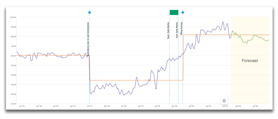
Figure 4 – Forecasting Example
As has been discussed, our ability to better interpret historical asset behavior has been hugely augmented in recent years with advancements in geospatial analytical platforms. Going well beyond the basic rendering of raw data sets, we are now able to leverage interpretation techniques such as smoothing and even event-based changes at a given point in time.
The real benefit though of these advancements is the enablement of better forecasting. Forecasts can now be generated in the context of historical patterns. Patterns not only from the asset in question itself but from other analogous assets as well.
The next step in this evolution of analysis will be to capture the actual performance of assets as they progress through their lifecycle and use this to validate, and more importantly, calibrate as needed, our forecasting techniques for future analysis and monitoring. A far cry from, but still keeping true to, the centuries-old principles and usage of a level and staff! If we can better track and interpret asset behavior, we have a much better chance of building and maintaining stronger, more efficient, and safer infrastructure.